Visualizing GPS data in R

2014-02-05 2 min read

Earlier today I read Nathan Yau’s post that had a quick R script to plot GPX file data onto a map. I was able to quickly load up my RunKeeper data from 2013 and came up with a pretty cool visualization of each of my outdoor runs. Since my runs occurred across multiple cities and continents the visualization turned out to be very sparse without a great sense of where the runs were. I made a two quick changes to the script to make it more useful for my data: a map overlay to see where in the world I ran and an ability to view a zoomed in area of the map. I’ve included the updated script and the resulting plots below.

# From Nathan's script
library(plotKML)
library(ggplot2)
library(maps)

# GPX files downloaded from Runkeeper
files <- dir(pattern = "\\.gpx")

# Consolidate routes in one drata frame
index <- c()
lat <- c()
long <- c()
for (i in 1:length(files)) {

  route <- readGPX(files[i])
  location <- route$tracks[[1]][[1]]

  index <- c(index, rep(i, dim(location)[1]))
  lat <- c(lat, location$lat)
  long <- c(long, location$lon)
}
routes <- data.frame(cbind(index, lat, long))

# Map the routes
ids <- unique(index)
plot(routes$long, routes$lat, type="n", axes=FALSE, xlab="", ylab="", main="", asp=1)
for (i in 1:length(ids)) {
  currRoute <- subset(routes, index==ids[i])
  lines(currRoute$long, currRoute$lat, col="#FF000020")
}

# Add the world map overlay
world <- map_data('world')
plot(world$long, world$lat, type="n", axes=FALSE, xlab="", ylab="", main="", asp=1)

world_groups <- unique(world$group)
for (i in 1:length(world_groups)) {
  currRoute <- subset(world, group==world_groups[i])
  lines(currRoute$long, currRoute$lat, col="#00000020")
}

route_groups <- unique(routes$index)
for (i in 1:length(route_groups)) {
  currRoute <- subset(routes, index==route_groups[i])
  lines(currRoute$long, currRoute$lat, col="#FF000020")
}

# Zoom into a particular area of routes
zoom <- function(routes, lat, long, radius) {
  lat_north <- lat + radius
  long_west <- long - radius
  lat_south <- lat - radius
  long_east <- long + radius
  routes.filtered <- routes[routes$lat < lat_north & routes$lat > lat_south & routes$long > long_west & routes$long < long_east, ]

  plot(routes.filtered$long, routes.filtered$lat, type="n", axes=FALSE, xlab="", ylab="", main="", asp=1)
  route_groups <- unique(routes.filtered$index)
  for (i in 1:length(route_groups)) {
    currRoute <- subset(routes.filtered, index==route_groups[i])
    lines(currRoute$long, currRoute$lat, col="#FF000020")
  }
}

hoboken_lat <- 40.79
hoboken_long <- -74.0279
radius <- 0.25

zoom(routes, hoboken_lat, hoboken_long, radius)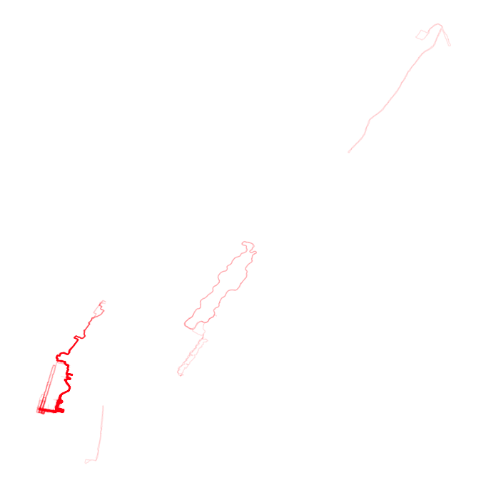

A few specks here and there - clearly visible runs in the NY/NJ area as well as some in Virginia, New Orleans, and San Francisco. Can also see a few runs in India.
Zoom in on my runs in the Hoboken/NYC area. I don't have the lat/long coordinates here but if I had them it would be pretty easy to generate a map overlay.

Dan Goldin

Visualizing GPS data in R